7 Pareto Analysis for Quality Improvement
7.1 Learning Objectives
By the end of this chapter, you will:
- Create and interpret Pareto charts using the qcc package
- Apply the 80/20 principle to quality problems
- Use Pareto analysis for prioritizing improvement efforts
- Connect Pareto analysis to control chart data
- Design data-driven improvement strategies
7.2 Introduction to Pareto Analysis
Pareto analysis30 is one of the most powerful tools in quality improvement. Named after Italian economist Vilfredo Pareto, it’s built on the principle that 80% of problems come from 20% of causes.
Think of Pareto analysis as your quality improvement compass—it points you toward the few critical issues that will give you the biggest improvement impact for your effort.
7.2.1 The Pareto Principle (80/20 Rule)
The Pareto principle suggests that in many situations:
- 80% of defects come from 20% of causes
- 80% of customer complaints come from 20% of issues
- 80% of costs come from 20% of problems
- 80% of improvement potential lies in 20% of areas
The Power of Focus
Instead of spreading your improvement efforts thin across many small issues, Pareto analysis helps you focus on the “vital few” problems that will deliver the greatest impact.
7.3 Creating Pareto Charts with QCC
7.3.1 Basic Pareto Chart
Let’s start with a simple example of defects in a manufacturing process:
# Manufacturing defect data
defects <- c(85, 45, 38, 32, 28, 18, 12, 8)
names(defects) <- c("Scratches", "Dents", "Wrong Color", "Size Issue",
                    "Missing Parts", "Cracks", "Rough Surface", "Other")

# Create Pareto chart
pc <- qcc::pareto.chart(defects, ylab = "Defect Count",
                      main = "Manufacturing Defects Analysis")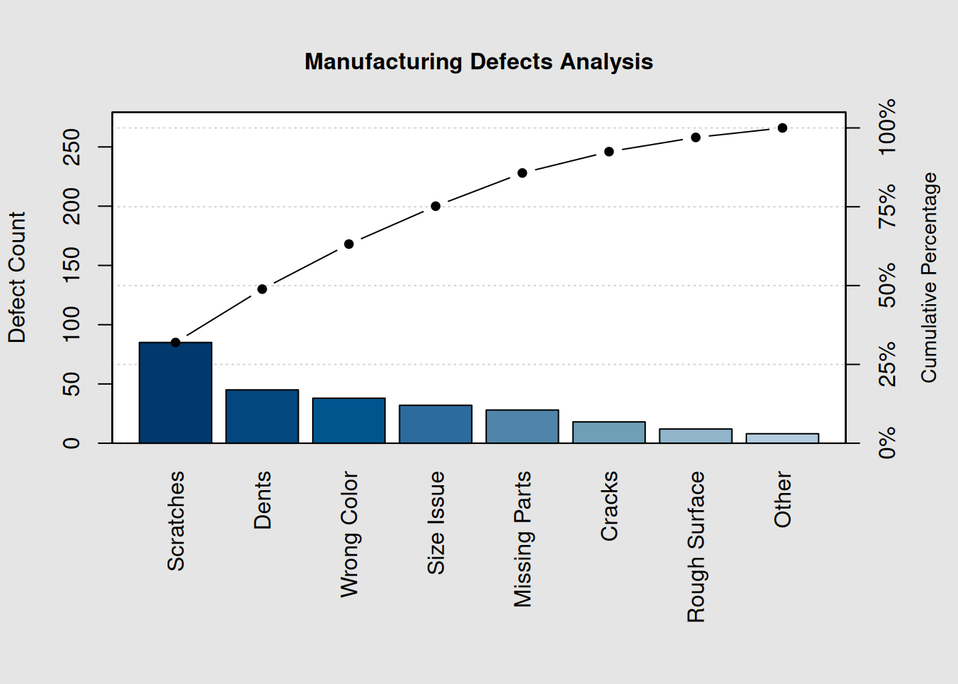
print(pc)##
## Pareto chart analysis for defects
## Frequency Cum.Freq. Percentage Cum.Percent.
## Scratches 85.000000 85.000000 31.954887 31.954887
## Dents 45.000000 130.000000 16.917293 48.872180
## Wrong Color 38.000000 168.000000 14.285714 63.157895
## Size Issue 32.000000 200.000000 12.030075 75.187970
## Missing Parts 28.000000 228.000000 10.526316 85.714286
## Cracks 18.000000 246.000000 6.766917 92.481203
## Rough Surface 12.000000 258.000000 4.511278 96.992481
## Other 8.000000 266.000000 3.007519 100.0000007.3.2 Understanding the Pareto Chart
The chart shows: 1. Bars: Defect frequencies in descending order 2. Line: Cumulative percentage of total defects 3. 80% line: Visual reference for the 80/20 rule
# Extract the most critical categories (contributing to ~80% of problems)
cumulative_pct <- pc[, "Cum.Percent."]
critical_categories <- names(cumulative_pct[cumulative_pct <= 80])

cat("Critical Categories (80% of problems):\n")
## Critical Categories (80% of problems):## 1. Scratches
## 2. Dents
## 3. Wrong Color
## 4. Size Issue7.4 Real-World Pareto Analysis Examples
7.4.1 Example 1: Customer Complaints
# Customer complaint data from service center
complaints <- c(156, 89, 67, 45, 33, 28, 21, 18, 14, 9)
names(complaints) <- c("Long Wait Time", "Rude Staff", "Wrong Information",
                      "System Down", "No Follow-up", "Billing Error",
                      "Poor Communication", "Facility Issues",
                      "Limited Hours", "Other")

# Create Pareto chart
pc_complaints <- qcc::pareto.chart(complaints,
                                 ylab = "Number of Complaints",
                                 main = "Customer Complaints Analysis")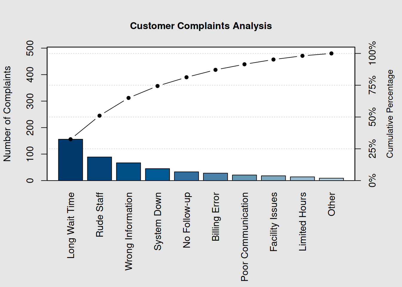
# Calculate improvement impact
total_complaints <- sum(complaints)
top_3_impact <- sum(complaints[1:3])
improvement_potential <- round((top_3_impact / total_complaints) * 100, 1)

cat("Total complaints:", total_complaints, "\n")
## Total complaints: 480
cat("Top 3 categories represent:", improvement_potential, "% of all complaints\n")## Top 3 categories represent: 65 % of all complaints7.4.2 Example 2: Process Downtime Analysis
# Manufacturing downtime data (hours per month)
downtime <- c(24, 18, 15, 12, 8, 6, 4, 3, 2, 1)
names(downtime) <- c("Equipment Failure", "Material Shortage", "Changeover Time",
                    "Quality Issues", "Maintenance", "Power Outage",
                    "Operator Absence", "Tool Wear", "Computer Issue", "Other")

# Create enhanced Pareto chart with custom colors
colors <- c("red", "orange", "yellow", rep("lightblue", 7))
pc_downtime <- qcc::pareto.chart(downtime,
                               ylab = "Downtime Hours",
                               main = "Monthly Process Downtime Analysis")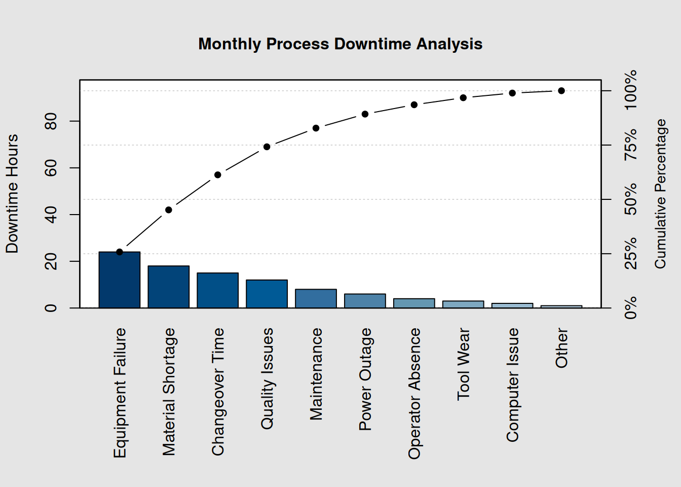
# Cost impact analysis
cost_per_hour <- 500  # Cost per downtime hour
total_cost <- sum(downtime) * cost_per_hour
vital_few_cost <- sum(downtime[1:3]) * cost_per_hour

cat("Total monthly downtime cost: $", format(total_cost, big.mark = ","), "\n", sep = "")
## Total monthly downtime cost: $46,500## Top 3 causes cost: $28,500
cat("Potential savings from addressing top 3: ",
    round((vital_few_cost/total_cost)*100, 1), "%\n", sep = "")
## Potential savings from addressing top 3: 61.3%7.5 80/20 Principle Application in Quality
7.5.1 Identifying the Vital Few
# Function to identify vital few categories
identify_vital_few <- function(data, threshold = 80) {
  # Sort data in descending order
  sorted_data <- sort(data, decreasing = TRUE)

  # Calculate cumulative percentage
  total <- sum(sorted_data)
  cumulative <- cumsum(sorted_data)
  cum_percent <- (cumulative / total) * 100

  # Find vital few (categories contributing to threshold%)
  vital_few_count <- sum(cum_percent <= threshold)

  # Handle case where first category exceeds threshold
  if(vital_few_count == 0) vital_few_count <- 1

  vital_few <- names(sorted_data)[1:vital_few_count]
  vital_few_contribution <- cum_percent[vital_few_count]

  return(list(
    categories = vital_few,
    count = vital_few_count,
    contribution = round(vital_few_contribution, 1),
    total_categories = length(data)
  ))
}

# Apply to our defects example
vf <- identify_vital_few(defects)
cat("Vital Few Analysis:\n")
## Vital Few Analysis:
cat("Categories analyzed:", vf$total_categories, "\n")## Categories analyzed: 8## Vital few categories: 4 ( 50 %)
cat("Their contribution:", vf$contribution, "% of total problems\n")## Their contribution: 75.2 % of total problems
cat("\nThe vital few are:\n")##
## The vital few are:## - Scratches
## - Dents
## - Wrong Color
## - Size Issue7.5.2 Before and After Improvement
# Simulating improvement after addressing top issues
defects_before <- defects
defects_after <- defects_before

# Simulate 70% reduction in top 3 categories after improvement
defects_after[1:3] <- round(defects_after[1:3] * 0.3)

# Create comparison data
comparison_data <- data.frame(
  Category = names(defects),
  Before = as.numeric(defects_before),
  After = as.numeric(defects_after),
  Reduction = defects_before - defects_after
)

# Sort by reduction achieved
comparison_data <- comparison_data[order(-comparison_data$Reduction), ]

cat("Improvement Impact Analysis:\n")
## Improvement Impact Analysis:## Total defects before: 266## Total defects after: 149
cat("Overall reduction:", sum(defects_before) - sum(defects_after),
    "(", round(((sum(defects_before) - sum(defects_after))/sum(defects_before))*100, 1), "%)\n\n")
## Overall reduction: 117 ( 44 %)
print(comparison_data[1:5, ]) # Show top 5 improvements## Category Before After Reduction
## Scratches Scratches 85 26 59
## Dents Dents 45 14 31
## Wrong Color Wrong Color 38 11 27
## Size Issue Size Issue 32 32 0
## Missing Parts Missing Parts 28 28 07.6 Prioritizing Improvement Efforts
7.6.1 Multi-Criteria Pareto Analysis
Sometimes you need to consider multiple factors beyond just frequency:
# Quality issues with multiple impact factors
quality_issues <- data.frame(
  Issue = c("Surface Defects", "Dimensional Error", "Material Flaw",
           "Assembly Issue", "Packaging Problem", "Label Error"),
  Frequency = c(45, 38, 32, 28, 18, 12),
  Cost_Impact = c(150, 200, 300, 120, 50, 25),  # Cost per occurrence
  Customer_Impact = c(3, 5, 4, 2, 1, 1)  # Severity scale 1-5
)

# Calculate weighted impact score
quality_issues$Total_Cost <- quality_issues$Frequency * quality_issues$Cost_Impact
quality_issues$Weighted_Score <- quality_issues$Total_Cost * quality_issues$Customer_Impact

# Create Pareto chart based on weighted score
weighted_scores <- quality_issues$Weighted_Score
names(weighted_scores) <- quality_issues$Issue

pc_weighted <- qcc::pareto.chart(weighted_scores,
                               ylab = "Weighted Impact Score",
                               main = "Multi-Criteria Quality Issues Analysis")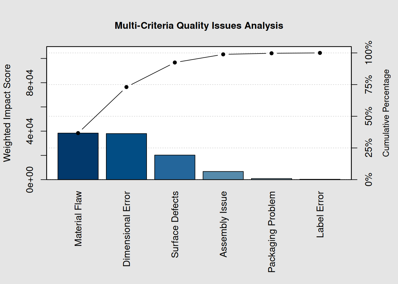
# Show the analysis table
cat("Multi-Criteria Analysis:\n")
## Multi-Criteria Analysis:## Issue Frequency Cost_Impact Customer_Impact Total_Cost
## 3 Material Flaw 32 300 4 9600
## 2 Dimensional Error 38 200 5 7600
## 1 Surface Defects 45 150 3 6750
## 4 Assembly Issue 28 120 2 3360
## 5 Packaging Problem 18 50 1 900
## 6 Label Error 12 25 1 300
## Weighted_Score
## 3 38400
## 2 38000
## 1 20250
## 4 6720
## 5 900
## 6 3007.6.2 Action Priority Matrix
# Create action priority recommendations
create_priority_matrix <- function(data) {
  # Rank categories by impact (1 = highest impact)
  ranked_data <- data[order(-data)]
  n_categories <- length(ranked_data)

  # Simple priority classification
  priorities <- character(n_categories)
  priorities[1:ceiling(n_categories*0.2)] <- "HIGH"
  priorities[(ceiling(n_categories*0.2)+1):ceiling(n_categories*0.5)] <- "MEDIUM"
  priorities[(ceiling(n_categories*0.5)+1):n_categories] <- "LOW"

  # Create recommendations
  recommendations <- character(n_categories)
  recommendations[priorities == "HIGH"] <- "Address immediately - major impact"
  recommendations[priorities == "MEDIUM"] <- "Schedule for next phase"
  recommendations[priorities == "LOW"] <- "Monitor and address if resources allow"

  return(data.frame(
    Category = names(ranked_data),
    Impact_Value = as.numeric(ranked_data),
    Priority = priorities,
    Recommendation = recommendations,
    stringsAsFactors = FALSE
  ))
}

# Apply to our complaints example
priority_matrix <- create_priority_matrix(complaints)
cat("Action Priority Matrix:\n")
## Action Priority Matrix:
print(priority_matrix)## Category Impact_Value Priority
## 1 Long Wait Time 156 HIGH
## 2 Rude Staff 89 HIGH
## 3 Wrong Information 67 MEDIUM
## 4 System Down 45 MEDIUM
## 5 No Follow-up 33 MEDIUM
## 6 Billing Error 28 LOW
## 7 Poor Communication 21 LOW
## 8 Facility Issues 18 LOW
## 9 Limited Hours 14 LOW
## 10 Other 9 LOW
## Recommendation
## 1 Address immediately - major impact
## 2 Address immediately - major impact
## 3 Schedule for next phase
## 4 Schedule for next phase
## 5 Schedule for next phase
## 6 Monitor and address if resources allow
## 7 Monitor and address if resources allow
## 8 Monitor and address if resources allow
## 9 Monitor and address if resources allow
## 10 Monitor and address if resources allow7.7 Connecting Pareto Analysis to Control Charts
7.7.1 From Control Chart Signals to Pareto Analysis
# Simulate control chart violation data
violation_types <- c("Point beyond limits", "Two of three beyond 2-sigma",
                    "Four of five beyond 1-sigma", "Eight consecutive on one side",
                    "Six consecutive increasing", "Fifteen within 1-sigma",
                    "Eight beyond 1-sigma")

# Simulate frequencies of different violation types
violations <- c(28, 15, 12, 18, 8, 5, 3)
names(violations) <- violation_types

# Create Pareto chart for control chart violations
pc_violations <- qcc::pareto.chart(violations,
                                 ylab = "Frequency of Violations",
                                 main = "Control Chart Violation Analysis")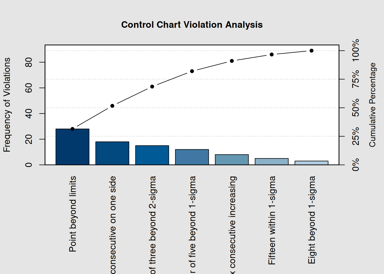
cat("Control Chart Investigation Priority:\n")## Control Chart Investigation Priority:
cat("Most common violations require immediate attention:\n")## Most common violations require immediate attention:
top_violations <- names(sort(violations, decreasing = TRUE)[1:3])
for(i in 1:length(top_violations)) {
  cat(i, ". ", top_violations[i], "\n", sep = "")
}
## 1. Point beyond limits
## 2. Eight consecutive on one side
## 3. Two of three beyond 2-sigma7.7.2 Root Cause Integration
# Connect Pareto findings to root cause categories
root_causes <- c("Machine", "Method", "Material", "Manpower", "Measurement", "Environment")
cause_frequency <- c(42, 35, 28, 18, 12, 8)
names(cause_frequency) <- root_causes

# Create root cause Pareto
pc_causes <- qcc::pareto.chart(cause_frequency,
                             ylab = "Root Cause Frequency",
                             main = "Root Cause Analysis - 6M Categories")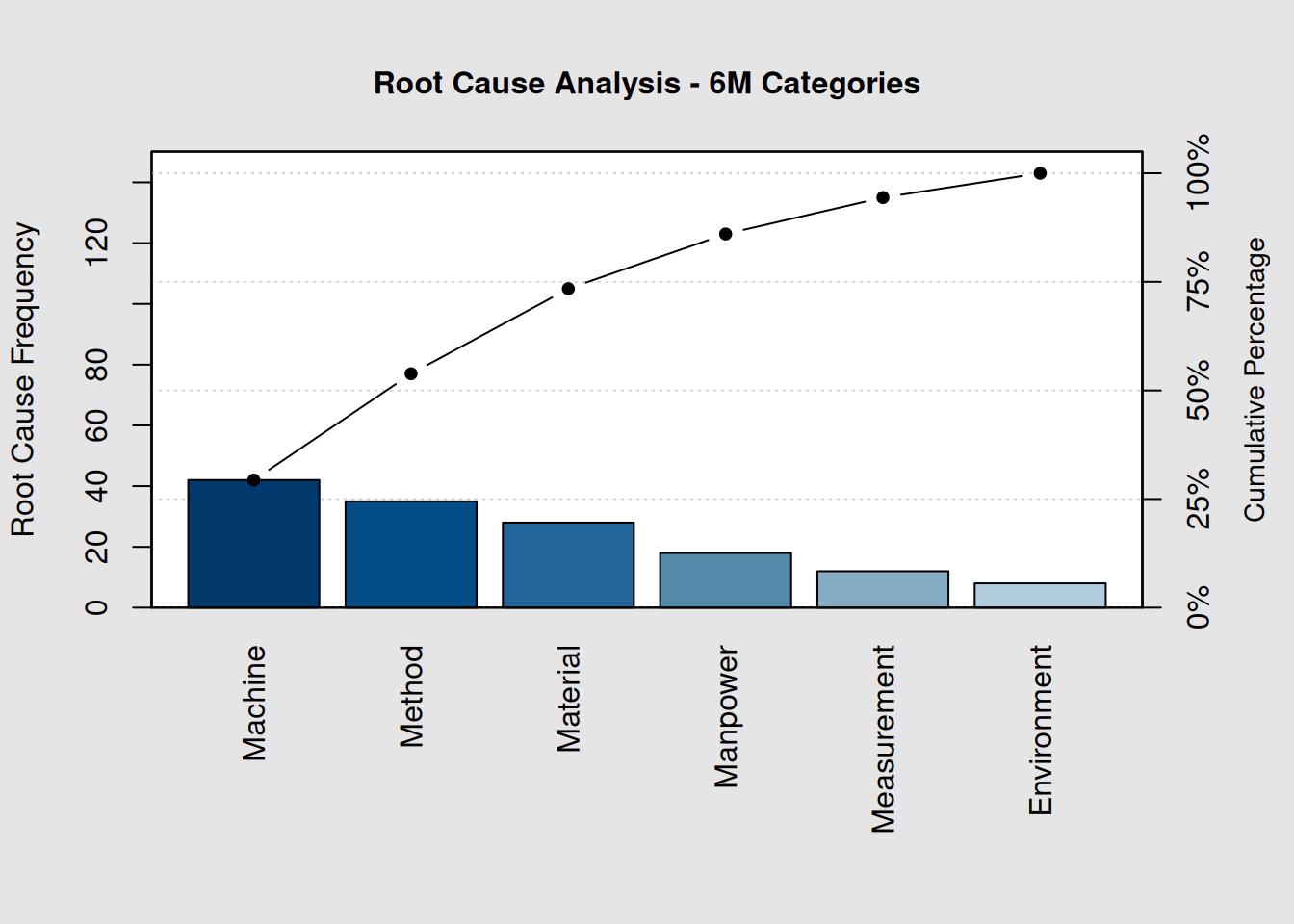
# Calculate focus areas for improvement teams
vital_causes <- names(sort(cause_frequency, decreasing = TRUE)[1:3])
cat("Primary focus areas for improvement teams:\n")
## Primary focus areas for improvement teams:## 1. Machine issues
## 2. Method issues
## 3. Material issues7.8 Data Collection Strategies for Pareto Analysis
7.8.1 Designing Data Collection Systems
Effective Data Collection for Pareto Analysis
-
Standardize Categories: Use consistent, specific category definitions
-
Train Data Collectors: Ensure consistent classification of issues
-
Capture Context: Include time, location, operator information
-
Regular Updates: Refresh analysis as improvements are implemented
-
Multiple Perspectives: Consider frequency, cost, and customer impact
# Example of structured data collection
quality_log <- data.frame(
  Date = rep(c("2024-01-15", "2024-01-16", "2024-01-17"), each = 10),
  Shift = rep(c("A", "B", "C"), 10),
  Defect_Type = sample(names(defects), 30, replace = TRUE,
                      prob = defects/sum(defects)),
  Operator = sample(c("Operator1", "Operator2", "Operator3", "Operator4"), 30, replace = TRUE),
  Cost_Impact = sample(c(25, 50, 75, 100), 30, replace = TRUE)
)

# Analyze by different dimensions
cat("Pareto by Defect Type:\n")
## Pareto by Defect Type:##
## Scratches Dents Size Issue Rough Surface Cracks
## 6 5 5 4 3
## Wrong Color Missing Parts Other
## 3 2 2
cat("\nPareto by Shift:\n") ##
## Pareto by Shift:##
## A B C
## 10 10 10
cat("\nPareto by Operator:\n")##
## Pareto by Operator:##
## Operator4 Operator2 Operator3 Operator1
## 11 10 5 47.9 Advanced Pareto Techniques
7.9.1 Time-Based Pareto Analysis
# Monthly defect trends
months <- c("Jan", "Feb", "Mar", "Apr", "May", "Jun")
monthly_defects <- list(
  Jan = c(45, 32, 28, 20, 15),
  Feb = c(38, 35, 30, 18, 12),
  Mar = c(42, 30, 25, 22, 10),
  Apr = c(35, 28, 22, 15, 8),
  May = c(30, 25, 20, 12, 6),
  Jun = c(28, 22, 18, 10, 5)
)

defect_types <- c("Scratches", "Dents", "Wrong Color", "Size Issue", "Missing Parts")
names(monthly_defects$Jan) <- defect_types
names(monthly_defects$Feb) <- defect_types
names(monthly_defects$Mar) <- defect_types
names(monthly_defects$Apr) <- defect_types
names(monthly_defects$May) <- defect_types
names(monthly_defects$Jun) <- defect_types

# Show trend in top defect category
cat("Trend Analysis - Top Defect Category (Scratches):\n")
## Trend Analysis - Top Defect Category (Scratches):
scratches_trend <- sapply(monthly_defects, function(x) x["Scratches"])
cat("Jan:", scratches_trend[1], " Feb:", scratches_trend[2],
    " Mar:", scratches_trend[3], " Apr:", scratches_trend[4],
    " May:", scratches_trend[5], " Jun:", scratches_trend[6], "\n")
## Jan: 45 Feb: 38 Mar: 42 Apr: 35 May: 30 Jun: 28
# Calculate improvement rate
improvement_rate <- round(((scratches_trend[1] - scratches_trend[6]) / scratches_trend[1]) * 100, 1)
cat("Improvement in Scratches:", improvement_rate, "%\n")
## Improvement in Scratches: 37.8 %7.9.2 Stratified Pareto Analysis
# Pareto analysis by product line
product_a_defects <- c(25, 18, 15, 12, 8)
product_b_defects <- c(30, 20, 10, 8, 5)
product_c_defects <- c(20, 15, 18, 10, 12)

names(product_a_defects) <- defect_types
names(product_b_defects) <- defect_types
names(product_c_defects) <- defect_types

cat("Stratified Pareto Analysis by Product Line:\n\n")
## Stratified Pareto Analysis by Product Line:
cat("Product A - Top 3 Issues:\n")## Product A - Top 3 Issues:
top_a <- names(sort(product_a_defects, decreasing = TRUE)[1:3])
for(i in 1:3) cat(i, ". ", top_a[i], "\n", sep = "")
## 1. Scratches
## 2. Dents
## 3. Wrong Color
cat("\nProduct B - Top 3 Issues:\n")##
## Product B - Top 3 Issues:
top_b <- names(sort(product_b_defects, decreasing = TRUE)[1:3])
for(i in 1:3) cat(i, ". ", top_b[i], "\n", sep = "")
## 1. Scratches
## 2. Dents
## 3. Wrong Color
cat("\nProduct C - Top 3 Issues:\n")##
## Product C - Top 3 Issues:
top_c <- names(sort(product_c_defects, decreasing = TRUE)[1:3])
for(i in 1:3) cat(i, ". ", top_c[i], "\n", sep = "")
## 1. Scratches
## 2. Wrong Color
## 3. Dents
# Find common issues across products
common_issues <- intersect(intersect(top_a, top_b), top_c)
cat("\nCommon issues across all products:\n")
##
## Common issues across all products:
if(length(common_issues) > 0) {
  for(issue in common_issues) cat("- ", issue, "\n", sep = "")
} else {
  cat("No common issues in top 3 across all products\n")
}
## - Scratches
## - Dents
## - Wrong Color7.10 Implementation Best Practices
7.10.1 Step-by-Step Implementation Guide
-
Define the Problem
- Clearly specify what you’re analyzing
- Set measurement boundaries and timeframe
- Identify data sources
- Clearly specify what you’re analyzing
-
Collect Data
- Use standardized data collection methods
- Ensure sufficient sample size
- Include relevant stratification factors
- Use standardized data collection methods
-
Create Pareto Chart
- Sort data in descending order
- Calculate cumulative percentages
- Identify the vital few (typically 20% of categories)
- Sort data in descending order
-
Analyze Results
- Focus on categories contributing to 80% of problems
- Consider multiple criteria (frequency, cost, impact)
- Look for patterns and trends
- Focus on categories contributing to 80% of problems
-
Prioritize Actions
- Start with highest-impact items
- Consider resource requirements
- Set realistic timelines
- Start with highest-impact items
-
Implement and Monitor
- Address vital few categories first
- Track progress with updated Pareto charts
- Adjust priorities as improvements take effect
- Address vital few categories first
7.10.2 Common Pitfalls to Avoid
Pareto Analysis Pitfalls
-
Over-relying on frequency alone - Consider cost and customer impact
-
Static analysis - Update regularly as conditions change
-
Too many categories - Consolidate similar issues for clarity
-
Ignoring the “trivial many” - They may indicate systemic issues
-
Analysis paralysis - Start acting on clear priorities
7.11 Pareto Analysis Success Stories
7.11.1 Manufacturing Example
# Before improvement initiative
defects_baseline <- c(85, 45, 38, 32, 28, 18, 12, 8)
names(defects_baseline) <- c("Scratches", "Dents", "Wrong Color", "Size Issue",
                            "Missing Parts", "Cracks", "Rough Surface", "Other")

# After 6-month focused improvement on top 3 issues
defects_improved <- defects_baseline
defects_improved[1:3] <- round(defects_improved[1:3] * 0.25)  # 75% reduction

# Calculate business impact
total_reduction <- sum(defects_baseline) - sum(defects_improved)
cost_per_defect <- 45  # Average cost per defect
annual_savings <- total_reduction * cost_per_defect * 12  # Monthly to annual

cat("Manufacturing Improvement Success Story:\n")
## Manufacturing Improvement Success Story:## Baseline total defects: 266## Improved total defects: 140
cat("Monthly reduction:", total_reduction, "defects\n")## Monthly reduction: 126 defects## Estimated annual savings: $68,040
cat("ROI focus: Addressed only", sum(defects_baseline[1:3] > 0), "categories (",
    round((3/length(defects_baseline))*100, 0), "%) for maximum impact\n")
## ROI focus: Addressed only 3 categories ( 38 %) for maximum impact7.12 Integration with Other Quality Tools
7.12.1 Pareto + Control Charts
cat("Integrating Pareto Analysis with Control Charts:\n\n")## Integrating Pareto Analysis with Control Charts:
cat("1. Use Control Charts to detect when problems occur\n")## 1. Use Control Charts to detect when problems occur
cat("2. Use Pareto Analysis to identify which problems to solve first\n") ## 2. Use Pareto Analysis to identify which problems to solve first
cat("3. Focus improvement efforts on vital few categories\n")## 3. Focus improvement efforts on vital few categories
cat("4. Monitor with Control Charts to verify improvements\n")## 4. Monitor with Control Charts to verify improvements
cat("5. Update Pareto Analysis to find next priorities\n\n")## 5. Update Pareto Analysis to find next priorities
cat("This creates a continuous improvement cycle:\n")## This creates a continuous improvement cycle:
cat("DETECT (Control Charts) → PRIORITIZE (Pareto) → IMPROVE → VERIFY → REPEAT\n")## DETECT (Control Charts) → PRIORITIZE (Pareto) → IMPROVE → VERIFY → REPEAT7.12.2 Pareto + Capability Studies
# Connect Pareto findings to capability improvement
cat("Using Pareto with Process Capability:\n\n")
## Using Pareto with Process Capability:
cat("When Cpk < 1.33:\n")## When Cpk < 1.33:
cat("1. Create Pareto chart of defect types\n")## 1. Create Pareto chart of defect types
cat("2. Focus capability improvement on vital few defects\n") ## 2. Focus capability improvement on vital few defects
cat("3. Address root causes of top categories\n")## 3. Address root causes of top categories
cat("4. Re-calculate capability after improvements\n")## 4. Re-calculate capability after improvements
cat("5. Repeat until Cpk ≥ 1.33\n\n")## 5. Repeat until Cpk ≥ 1.33
cat("This targeted approach is more efficient than general process improvements\n")## This targeted approach is more efficient than general process improvements7.13 Key Takeaways
-
Focus on the Vital Few: 80% of problems typically come from 20% of causes
-
Use Multiple Criteria: Consider frequency, cost, and customer impact
-
Act on Priorities: Start with highest-impact categories first
-
Monitor Progress: Update Pareto charts to track improvement
-
Integrate with Other Tools: Combine with control charts and capability studies
- Stratify Data: Analyze by different dimensions for deeper insights
7.14 Chapter Summary
Pareto analysis is a cornerstone of effective quality improvement. By identifying the vital few causes that create the majority of problems, you can focus your limited resources where they will have the greatest impact.
The power of Pareto analysis lies not just in the 80/20 principle, but in its ability to:
- Transform overwhelming problem lists into focused action plans
- Demonstrate improvement impact with clear before/after comparisons
- Guide resource allocation for maximum return on investment
- Integrate seamlessly with other quality tools like control charts
Remember: Pareto analysis is not a one-time activity. As you solve the vital few problems, new priorities will emerge. Regular updates to your Pareto analysis ensure your improvement efforts remain focused on the current critical issues.
This concludes our comprehensive QCC tutorial. You now have the knowledge to implement statistical process control, from basic control charts through advanced capability studies and improvement prioritization. Use these tools to drive meaningful quality improvements in your processes and create lasting value for your organization.