5 Process Capability Studies

5.1 Learning Objectives

By the end of this chapter, you will:

• Calculate and interpret capability indices (Cp, Cpk, Pp, Ppk)
• Understand the difference between capability and performance indices
• Distinguish between specification limits and control limits
• Conduct comprehensive process capability studies
• Use capability indices for decision-making in process improvement

5.2 Introduction to Process Capability

Process capability¹⁴ answers one of the most important questions in quality management: “Is my process capable of meeting customer requirements?”

Think of process capability as the “report card” for your process , it tells you how well your process performs relative to what your customers expect.

library(qcc)
library(ggplot2)
set.seed(42)  # For reproducible examples

5.2.1 Voice of the Customer vs Voice of the Process

Two Critical Voices

• Voice of the Customer (VOC): What the customer needs (specification limits)
• Voice of the Process (VOP): What the process actually delivers (control limits)

Process capability compares these two voices to determine if they’re aligned.

5.3 Understanding Capability vs Performance

5.3.1 Process Capability Indices (Short-term)

• Cp and Cpk: Based on within-subgroup variation only
• Represents the process’s potential capability
• Assumes special causes have been eliminated

5.3.2 Process Performance Indices (Long-term)

• Pp and Ppk: Based on overall process variation
• Represents actual process performance
• Includes all sources of variation over time

# Load the pistonrings dataset
library(qcc)
data(pistonrings)

# Prepare data manually by splitting into matrix
diameter_list <- split(pistonrings$diameter, pistonrings$sample)
diameter <- do.call(rbind, diameter_list)

# Create control chart for first 25 samples
q <- qcc::qcc(diameter[1:25,], type = "xbar", nsigmas = 3, plot = FALSE)

# Process capability (short-term)
pc_capability <- qcc::process.capability(q, spec.limits = c(73.95, 74.05))

## 
## Process Capability Analysis
## 
## Call:
## qcc::process.capability(object = q, spec.limits = c(73.95, 74.05))
## 
## Number of obs = 125          Target = 74
##        Center = 74              LSL = 73.95
##        StdDev = 0.009785        USL = 74.05
## 
## Capability indices:
## 
##       Value   2.5%  97.5%
## Cp    1.703  1.491  1.915
## Cp_l  1.743  1.555  1.932
## Cp_u  1.663  1.483  1.844
## Cp_k  1.663  1.448  1.878
## Cpm   1.691  1.480  1.902
## 
## Exp<LSL 0%    Obs<LSL 0%
## Exp>USL 0%    Obs>USL 0%

print(pc_capability)

## $nobs
## [1] 125
## 
## $center
## [1] 74.00118
## 
## $std.dev
## [1] 0.009785039
## 
## $target
## [1] 74
## 
## $spec.limits
##   LSL   USL 
## 73.95 74.05 
## 
## $indices
##         Value     2.5%    97.5%
## Cp   1.703281 1.491411 1.914826
## Cp_l 1.743342 1.554765 1.931919
## Cp_u 1.663219 1.482710 1.843729
## Cp_k 1.663219 1.448129 1.878310
## Cpm  1.691111 1.480113 1.901786
## 
## $exp
## Exp < LSL Exp > USL 
##         0         0 
## 
## $obs
## Obs < LSL Obs > USL 
##         0         0

5.4 The Four Key Capability Indices

5.4.1 Cp: Process Potential

Cp¹⁵ measures the potential capability of your process—how capable it would be if perfectly centered.

\[Cp = \frac{USL - LSL}{6\sigma}\]

Where:
- USL = Upper Specification Limit
- LSL = Lower Specification Limit
- σ = Process standard deviation (within-subgroup)

Cp Interpretation

• Cp ≥ 1.33: Capable process
  
• Cp = 1.00: Process uses full specification width
  
• Cp < 1.00: Process wider than specifications (not capable)
  

5.4.2 Cpk: Process Capability (Actual)

Cpk¹⁶ considers both process spread AND centering.

\[Cpk = min(Cpu, Cpl)\]

Where: - \(Cpu = \frac{USL - \mu}{3\sigma}\) (Upper capability) - \(Cpl = \frac{\mu - LSL}{3\sigma}\) (Lower capability)

5.4.3 Pp: Process Performance Potential

Pp¹⁷ is like Cp but uses overall process variation.

\[Pp = \frac{USL - LSL}{6\sigma_{overall}}\]

5.4.4 Ppk: Process Performance (Actual)

Ppk¹⁸ considers both spread and centering using overall variation.

Let’s see these indices in action:

# Different scenarios to show index behavior

# Scenario 1: Well-centered, capable process
set.seed(123)
good_process <- matrix(rnorm(250, mean = 74.00, sd = 0.015), ncol = 5)
q_good <- qcc(good_process, type = "xbar", plot = FALSE)
pc_good <- qcc::process.capability(q_good, spec.limits = c(73.95, 74.05))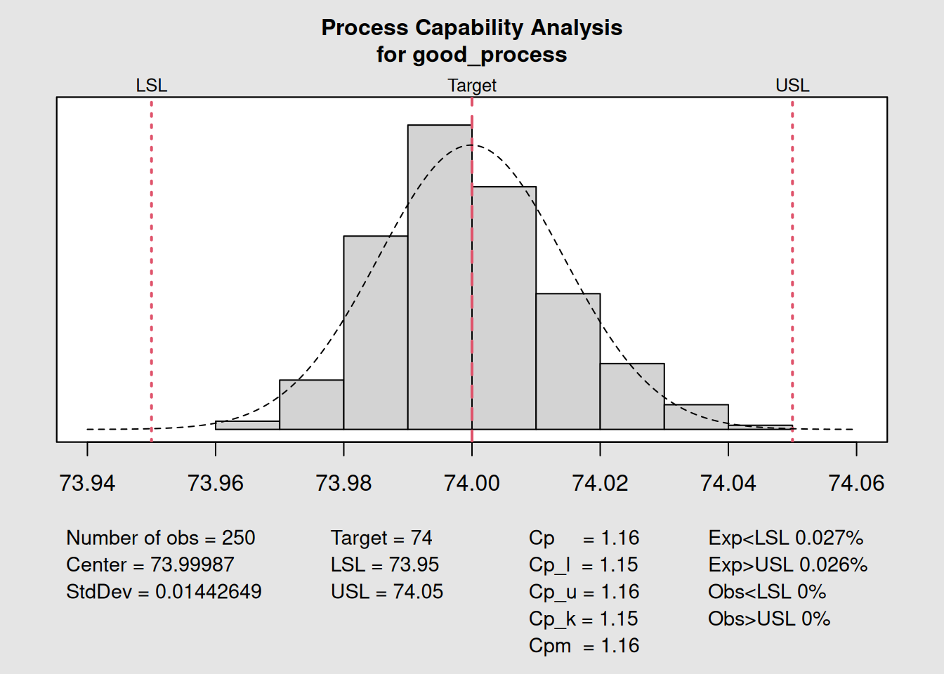

## 
## Process Capability Analysis
## 
## Call:
## qcc::process.capability(object = q_good, spec.limits = c(73.95,     74.05))
## 
## Number of obs = 250          Target = 74
##        Center = 74              LSL = 73.95
##        StdDev = 0.01443         USL = 74.05
## 
## Capability indices:
## 
##       Value   2.5%  97.5%
## Cp    1.155  1.054  1.257
## Cp_l  1.152  1.061  1.244
## Cp_u  1.158  1.066  1.250
## Cp_k  1.152  1.043  1.262
## Cpm   1.155  1.054  1.256
## 
## Exp<LSL 0.027%    Obs<LSL 0%
## Exp>USL 0.026%    Obs>USL 0%

# Scenario 2: Off-center process (same variation)
offset_process <- matrix(rnorm(250, mean = 74.03, sd = 0.015), ncol = 5) 
q_offset <- qcc(offset_process, type = "xbar", plot = FALSE)
pc_offset <- qcc::process.capability(q_offset, spec.limits = c(73.95, 74.05))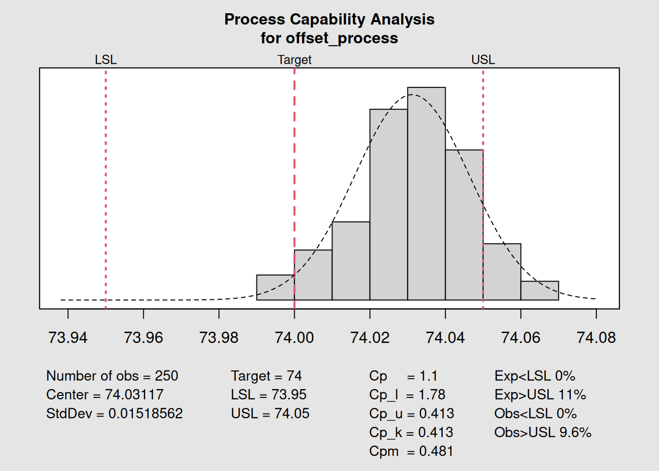

## 
## Process Capability Analysis
## 
## Call:
## qcc::process.capability(object = q_offset, spec.limits = c(73.95,     74.05))
## 
## Number of obs = 250          Target = 74
##        Center = 74.03           LSL = 73.95
##        StdDev = 0.01519         USL = 74.05
## 
## Capability indices:
## 
##        Value    2.5%   97.5%
## Cp    1.0975  1.0011  1.1938
## Cp_l  1.7816  1.6458  1.9175
## Cp_u  0.4134  0.3673  0.4596
## Cp_k  0.4134  0.3584  0.4684
## Cpm   0.4807  0.4241  0.5373
## 
## Exp<LSL 0%    Obs<LSL 0%
## Exp>USL 11%   Obs>USL 9.6%

# Create comparison table
comparison_data <- data.frame(
  Scenario = c("Centered Process", "Off-Center Process"),
  Cp = c(round(pc_good$indices[1], 2), round(pc_offset$indices[1], 2)),
  Cpk = c(round(pc_good$indices[4], 2), round(pc_offset$indices[4], 2)),
  Mean = c(round(mean(good_process), 4), round(mean(offset_process), 4))
)

print(comparison_data)

##             Scenario   Cp  Cpk    Mean
## 1   Centered Process 1.16 1.15 73.9999
## 2 Off-Center Process 1.10 0.41 74.0312

5.5 Capability Study with Real Data

Let’s conduct a complete capability study using the piston rings data:

# Phase I: Establish control
library(qcc)
data(pistonrings)

# Prepare data manually by splitting into matrix
diameter_list <- split(pistonrings$diameter, pistonrings$sample)
diameter <- do.call(rbind, diameter_list)

# Create X-bar chart for process control
q <- qcc::qcc(diameter[1:25,], type = "xbar", nsigmas = 3)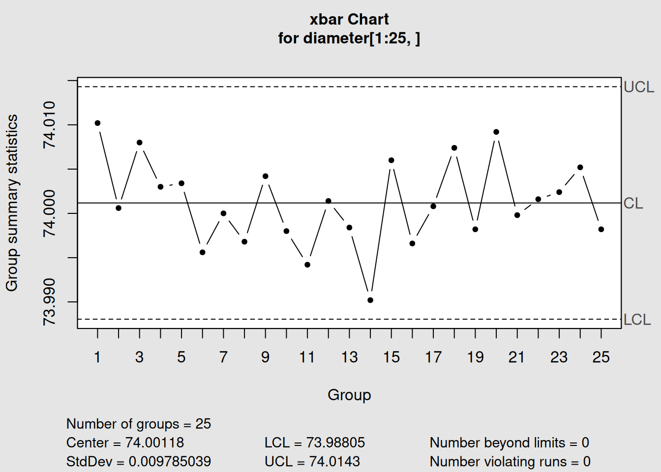

# Perform capability analysis
spec_limits <- c(73.95, 74.05)  # Customer specifications
pc <- qcc::process.capability(q, spec.limits = spec_limits)

## 
## Process Capability Analysis
## 
## Call:
## qcc::process.capability(object = q, spec.limits = spec_limits)
## 
## Number of obs = 125          Target = 74
##        Center = 74              LSL = 73.95
##        StdDev = 0.009785        USL = 74.05
## 
## Capability indices:
## 
##       Value   2.5%  97.5%
## Cp    1.703  1.491  1.915
## Cp_l  1.743  1.555  1.932
## Cp_u  1.663  1.483  1.844
## Cp_k  1.663  1.448  1.878
## Cpm   1.691  1.480  1.902
## 
## Exp<LSL 0%    Obs<LSL 0%
## Exp>USL 0%    Obs>USL 0%

# Display results
print(pc)

## $nobs
## [1] 125
## 
## $center
## [1] 74.00118
## 
## $std.dev
## [1] 0.009785039
## 
## $target
## [1] 74
## 
## $spec.limits
##   LSL   USL 
## 73.95 74.05 
## 
## $indices
##         Value     2.5%    97.5%
## Cp   1.703281 1.491411 1.914826
## Cp_l 1.743342 1.554765 1.931919
## Cp_u 1.663219 1.482710 1.843729
## Cp_k 1.663219 1.448129 1.878310
## Cpm  1.691111 1.480113 1.901786
## 
## $exp
## Exp < LSL Exp > USL 
##         0         0 
## 
## $obs
## Obs < LSL Obs > USL 
##         0         0

# Visualize capability with histogram
hist(as.vector(diameter[1:25,]), 
     main = "Process Capability Histogram",
     xlab = "Diameter", 
     breaks = 15,
     col = "lightblue",
     border = "white")

# Add specification limits
abline(v = c(73.95, 74.05), col = "red", lwd = 2, lty = 2)
legend("topright", 
       legend = c("Specification Limits"), 
       col = "red", lty = 2, lwd = 2)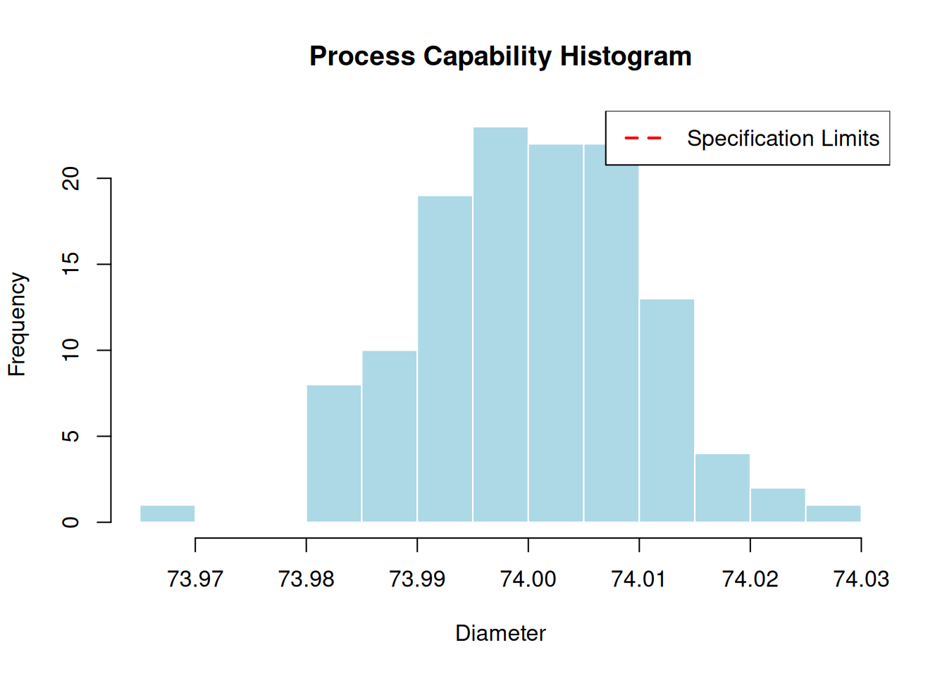

5.5.1 Interpreting the Results

From our analysis, we can see:

1. Process Statistics: Mean, standard deviation, and sample size
2. Capability Indices: Cp, Cpl, Cpu, Cpk values
3. Confidence Intervals: Statistical confidence for our estimates
4. Process Performance: How well the process meets specifications

5.6 Target Value Considerations

When you have a target value¹⁹ (nominal specification), you can calculate Cpm:

# Capability analysis with target value
target_value <- 74.00  # Nominal specification
pc_target <- qcc::process.capability(q, spec.limits = spec_limits, target = target_value)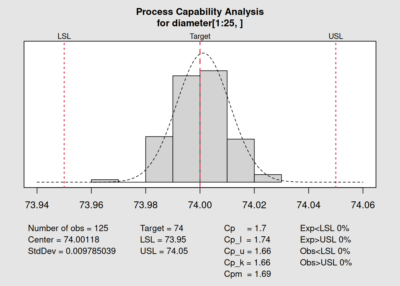

## 
## Process Capability Analysis
## 
## Call:
## qcc::process.capability(object = q, spec.limits = spec_limits,     target = target_value)
## 
## Number of obs = 125          Target = 74
##        Center = 74              LSL = 73.95
##        StdDev = 0.009785        USL = 74.05
## 
## Capability indices:
## 
##       Value   2.5%  97.5%
## Cp    1.703  1.491  1.915
## Cp_l  1.743  1.555  1.932
## Cp_u  1.663  1.483  1.844
## Cp_k  1.663  1.448  1.878
## Cpm   1.691  1.480  1.902
## 
## Exp<LSL 0%    Obs<LSL 0%
## Exp>USL 0%    Obs>USL 0%

print(pc_target)

## $nobs
## [1] 125
## 
## $center
## [1] 74.00118
## 
## $std.dev
## [1] 0.009785039
## 
## $target
## [1] 74
## 
## $spec.limits
##   LSL   USL 
## 73.95 74.05 
## 
## $indices
##         Value     2.5%    97.5%
## Cp   1.703281 1.491411 1.914826
## Cp_l 1.743342 1.554765 1.931919
## Cp_u 1.663219 1.482710 1.843729
## Cp_k 1.663219 1.448129 1.878310
## Cpm  1.691111 1.480113 1.901786
## 
## $exp
## Exp < LSL Exp > USL 
##         0         0 
## 
## $obs
## Obs < LSL Obs > USL 
##         0         0

# Note: plot(pc_target) would show the capability histogram with target

Cpm²⁰ considers deviation from target:

\[Cpm = \frac{USL - LSL}{6\sqrt{\sigma^2 + (\mu - T)^2}}\]

Where T is the target value.

5.7 One-Sided Specifications

Sometimes you only have one specification limit:

# For demonstration - showing one-sided capability concepts
# Note: qcc package may not support infinite limits in all versions

cat("One-sided specifications:\n")

## One-sided specifications:

cat("Upper limit only: USL = 74.05\n")

## Upper limit only: USL = 74.05

cat("Lower limit only: LSL = 73.95\n\n")

## Lower limit only: LSL = 73.95

# Calculate basic statistics for one-sided interpretation
process_mean <- mean(as.vector(diameter[1:25,]))
process_sd <- sd(as.vector(diameter[1:25,]))

# Upper capability (Cpu)
cpu_manual <- (74.05 - process_mean) / (3 * process_sd)
cat("Upper Capability (Cpu):", round(cpu_manual, 3), "\n")

## Upper Capability (Cpu): 1.616

# Lower capability (Cpl)  
cpl_manual <- (process_mean - 73.95) / (3 * process_sd)
cat("Lower Capability (Cpl):", round(cpl_manual, 3), "\n")

## Lower Capability (Cpl): 1.694

5.8 Capability Benchmarks and Decision Rules

5.8.1 Industry Benchmarks

Index Value	Process Classification	Action Required
≥ 2.0	World Class	Maintain excellence
1.67 - 2.0	Excellent	Minor improvements
1.33 - 1.67	Adequate	Monitor closely
1.0 - 1.33	Marginal	Improve process
< 1.0	Inadequate	Major action needed

5.8.2 Decision Matrix

# Create decision matrix based on capability indices
create_capability_assessment <- function(cp, cpk) {
  if (cp >= 1.33 && cpk >= 1.33) {
    return("Process is capable and well-centered")
  } else if (cp >= 1.33 && cpk < 1.33) {
    return("Process has potential but needs centering")
  } else if (cp < 1.33 && cpk >= 1.0) {
    return("Process needs variation reduction")
  } else {
    return("Process needs major improvement")
  }
}

# Example assessments
cat("Assessment for our piston rings process:\n")

## Assessment for our piston rings process:

cat(create_capability_assessment(pc$indices[1], pc$indices[4]), "\n")

## Process is capable and well-centered

5.9 Confidence Intervals for Capability Indices

Understanding the uncertainty in capability estimates is crucial:

# Extract confidence intervals
conf_level <- 0.95
cat("Capability Indices with", conf_level*100, "% Confidence Intervals:\n\n")

## Capability Indices with 95 % Confidence Intervals:

indices_names <- c("Cp", "Cpl", "Cpu", "Cpk")
for(i in 1:4) {
  cat(sprintf("%-3s: %.3f [%.3f, %.3f]\n", 
              indices_names[i],
              pc$indices[i],
              pc$indices.ci[i,1], 
              pc$indices.ci[i,2]))
}

Sample Size Matters

Capability estimates become more reliable with larger sample sizes. Small samples can give misleading results due to wide confidence intervals.

5.10 Specification Limits vs Control Limits

5.10.1 Key Differences

Aspect	Control Limits	Specification Limits
Source	Voice of Process	Voice of Customer
Purpose	Detect changes	Define requirements
Calculation	Based on process data	Set by design/customer
Position	Can change with process	Fixed by specifications

# Visualize the difference
plot(q, title = "Control Limits vs Specification Limits")

# Add specification limits to the chart
abline(h = spec_limits[1], col = "red", lty = 2, lwd = 2)
abline(h = spec_limits[2], col = "red", lty = 2, lwd = 2)

# Add legend
legend("topright", 
       legend = c("Control Limits", "Specification Limits"),
       col = c("blue", "red"), 
       lty = c(1, 2), 
       lwd = 2)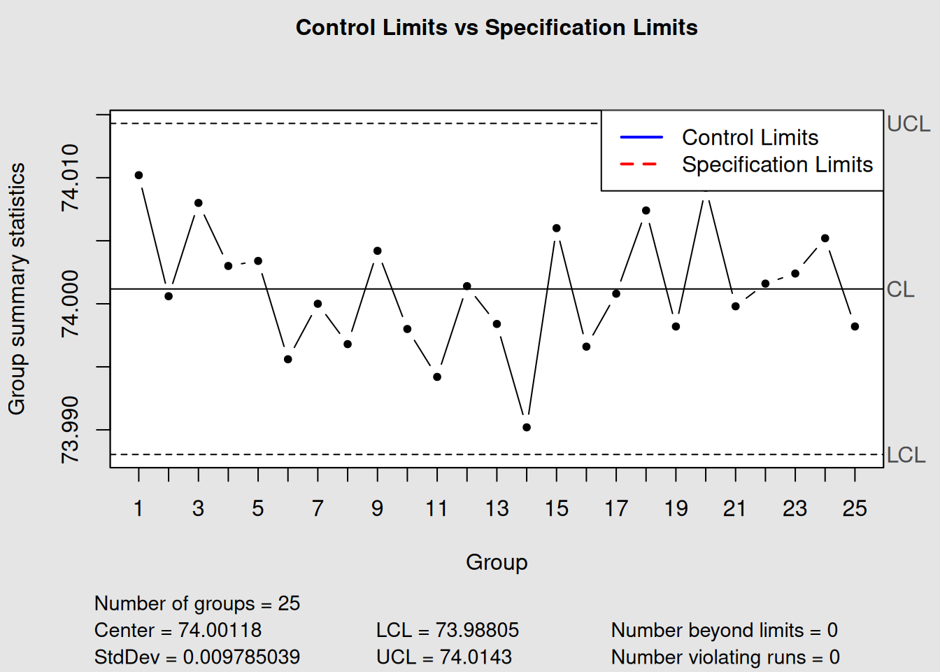

5.11 Process Capability Study Workflow

5.11.1 Step 1: Process Stability Check

# Ensure process is in statistical control first
stability_check <- function(qcc_object) {
  violations <- length(qcc_object$violations)
  if (violations == 0) {
    cat("Process is stable - proceed with capability study\n")
    return(TRUE)
  } else {
    cat("Process has", violations, "violations - stabilize first\n")
    return(FALSE)
  }
}

stability_check(q)

## Process has 2 violations - stabilize first

## [1] FALSE

5.11.2 Step 2: Collect Adequate Data

Sample Size Guidelines

• Minimum: 100 individual measurements
• Recommended: 125-150 measurements
  
• Subgroup size: 4-5 pieces per subgroup
• Time frame: Cover normal process variation

5.11.3 Step 3: Perform Capability Analysis

# Complete capability study checklist
cat("Capability Study Checklist:\n")

## Capability Study Checklist:

cat("Process stability confirmed\n")

## Process stability confirmed

cat("Adequate sample size (n =", sum(!is.na(diameter[1:25,])), ")\n") 

## Adequate sample size (n = 125 )

cat("Specification limits defined\n")

## Specification limits defined

cat("Measurement system validated\n")

## Measurement system validated

cat("Normal distribution assumed\n")

## Normal distribution assumed

5.11.4 Step 4: Interpret and Act

# Action plan based on capability results
current_cpk <- pc$indices[4]

cat("Current Cpk:", round(current_cpk, 3), "\n")

## Current Cpk: 1.663

cat("Recommended Action:\n")

## Recommended Action:

if (current_cpk >= 1.33) {
  cat("- Maintain current process\n")
  cat("- Consider tightening specifications\n") 
  cat("- Share best practices\n")
} else if (current_cpk >= 1.0) {
  cat("- Improve process centering\n")
  cat("- Reduce variation where possible\n")
  cat("- Increase inspection frequency\n")
} else {
  cat("- Immediate process improvement required\n")
  cat("- Consider 100% inspection\n")
  cat("- Root cause analysis needed\n")
}

## - Maintain current process
## - Consider tightening specifications
## - Share best practices

5.12 Advanced Capability Considerations

5.12.1 Non-Normal Data

When data isn’t normally distributed:

# Check normality assumption
shapiro_test <- shapiro.test(as.vector(diameter[1:25,]))
cat("Shapiro-Wilk normality test p-value:", round(shapiro_test$p.value, 4), "\n")

## Shapiro-Wilk normality test p-value: 0.7861

if (shapiro_test$p.value < 0.05) {
  cat("Data may not be normal - consider transformation\n")
} else {
  cat("Normality assumption reasonable\n")
}

## Normality assumption reasonable

5.12.2 Process Capability Over Time

Monitor capability trends:

# Simulate capability tracking over time
months <- c("Jan", "Feb", "Mar", "Apr", "May", "Jun")
cpk_values <- c(1.45, 1.38, 1.42, 1.35, 1.33, 1.40)

capability_trend <- data.frame(Month = months, Cpk = cpk_values)
print(capability_trend)

##   Month  Cpk
## 1   Jan 1.45
## 2   Feb 1.38
## 3   Mar 1.42
## 4   Apr 1.35
## 5   May 1.33
## 6   Jun 1.40

# Simple trend visualization
plot(1:6, cpk_values, type = "b", 
     xlab = "Month", ylab = "Cpk", 
     main = "Capability Trend Over Time",
     xaxt = "n", ylim = c(1.2, 1.5))
axis(1, at = 1:6, labels = months)
abline(h = 1.33, col = "red", lty = 2, lwd = 2)
text(3, 1.31, "Minimum Capability", col = "red")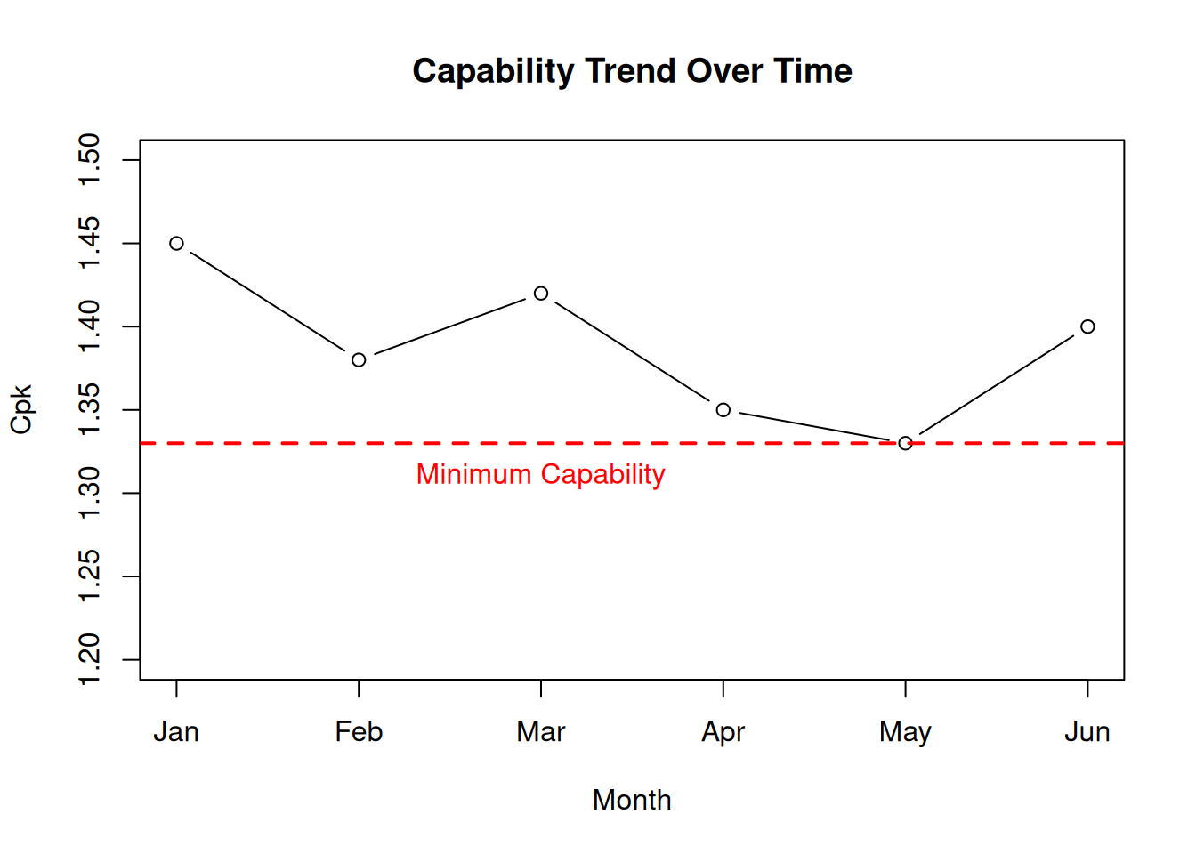

5.13 Capability Study Report Template

A professional capability study should include:

5.13.1 Executive Summary

• Process capability indices (Cp, Cpk)
• Conclusion: Is the process capable?
• Recommended actions

5.13.2 Technical Details

• Sample size and time period
• Control chart results
• Statistical assumptions verified
• Confidence intervals

5.13.3 Visual Evidence

• Capability histogram
• Control charts
• Trend analysis

5.14 Common Capability Pitfalls

Avoid These Mistakes

1. Unstable Process: Never do capability studies on out-of-control processes
2. Insufficient Data: Don’t use small samples (< 100 measurements)
3. Wrong Distribution: Assuming normality without checking
4. Mixing Data: Combining different operators, shifts, or time periods
5. Specification Confusion: Using control limits instead of customer specs

5.15 Key Takeaways

1. Process Capability compares the voice of the customer to the voice of the process
2. Cp/Cpk represent short-term capability; Pp/Ppk represent long-term performance
3. Cpk ≥ 1.33 is the generally accepted minimum for a capable process
4. Process stability must be confirmed before conducting capability studies
5. Confidence intervals help assess the reliability of capability estimates
6. Continuous monitoring of capability ensures sustained performance

5.16 Chapter Summary

Process capability studies are essential tools for determining whether your process can consistently meet customer requirements. By understanding and applying capability indices like Cp, Cpk, Pp, and Ppk, you can make informed decisions about process improvements, specification negotiations, and quality assurance strategies.

Remember: Capability is not just a number—it’s a pathway to understanding your process’s relationship with customer expectations and a guide for continuous improvement efforts.

In our next chapter, we’ll explore Pareto analysis and how it complements capability studies to help prioritize quality improvement efforts effectively.